CNN (Convolutional Neural Network)

011 min

The problem CNNs solve

Before CNNs, the natural way to feed an image into a neural network was to connect every pixel to every neuron in the next layer — a fully connected network. This falls apart quickly at the sizes real images come in. Connect one neuron to every pixel of a 100 by 100 image and that single neuron already needs 10,000 weights; a 1000 by 1000 color image needs 3 million weights per neuron. Stack a few layers and the parameter count becomes impossible to train or store.

There is a second, subtler problem. A fully connected network treats a pixel in the top-left corner and a pixel in the center as completely unrelated inputs. It has no built-in notion that pixels near each other are related, or that a cat is still a cat if it moves ten pixels to the right. So it has to learn, separately and from scratch, to recognize the same feature in every possible position — an enormous waste of data and capacity.

CNNs were designed to fix both problems at once. They exploit the fact that the useful patterns in an image are local — an edge is a small arrangement of nearby pixels — and that the same pattern can appear anywhere in the frame. That single insight is what makes vision tractable for a neural network.

022 min

How a CNN works

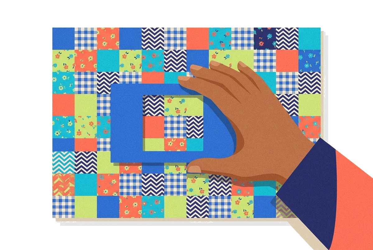
Follow one small filter — a 5 by 5 grid of weights that has learned to detect a vertical edge. Instead of giving each region of the image its own separate weights, the CNN slides this one filter across the whole image, computing at each position how strongly that patch looks like a vertical edge. This sliding operation is the convolution the network is named after, and its output is a feature map: a new image where bright spots mark where vertical edges were found.

This is where the efficiency comes from. Because the same filter is reused at every position, a convolutional layer processing 5 by 5 tiles needs only 25 weights, where a fully connected neuron on a 100 by 100 image needed 10,000. The network learns one edge detector and applies it everywhere, rather than relearning it for each location. The reused weights are also what let a CNN recognize a feature wherever it appears in the frame, because the same detector runs over every position.

After each convolution, a pooling layer shrinks the feature map by summarizing each small region down to a single value, usually its maximum. Pooling does two jobs: it cuts the data size for the next layer, and it grants a degree of local translational invariance, so a feature shifted by a pixel or two still registers. Stack these convolution-and-pooling blocks and the layers build up: the first detects edges, the next assembles edges into corners and textures, later ones assemble those into object parts, and a final fully connected layer turns the highest-level features into a classification. CNNs were inspired by biological vision — the connectivity pattern between their neurons resembles the organization of the animal visual cortex, where each neuron responds only to a small region of the visual field. The learned filters are trained the same way other networks are, by backpropagation.

031 min

A concrete example

The clearest checkable milestone is ImageNet, the standard image-classification benchmark of 1.2 million labeled photos across 1,000 categories. In 2012, AlexNet — a GPU-trained CNN by Alex Krizhevsky and colleagues — won the ImageNet Large Scale Visual Recognition Challenge, and the win was an early catalytic event for the modern AI boom. It was the moment CNNs went from a research curiosity to the dominant approach in computer vision.

The progress after that is easy to quantify on the same benchmark. In 2015, the ResNet architecture from Microsoft Research reported that an ensemble of its residual networks achieved 3.57% error on the ImageNet test set, winning first place on the ILSVRC 2015 classification task. That figure is below the commonly cited estimate of human top-5 error on the same task, which is why 2015 is often marked as the point where CNNs reached human-level accuracy on this specific benchmark. The number is real, tied to a named architecture, a named dataset, and a date — exactly the kind of claim that separates a measured result from a vague "CNNs are very accurate."

041 min

What CNNs mean for your work

For a product manager scoping an image feature — detecting defects on a production line, tagging user photos, reading receipts — a CNN is very often the right default, and this changes the plan concretely. CNNs need labeled training images, and the volume matters more than the model choice, so the honest first question is not "which architecture" but "can we get and label enough example images," because that, not the network, is usually what decides whether the feature ships.

For an engineer, the reusability of learned filters has a direct practical payoff: transfer learning. A CNN trained on ImageNet has already learned general-purpose edge and texture detectors in its early layers, and those transfer to a new task. Rather than train from scratch, an engineer can take a pretrained CNN and fine-tune it on a few thousand domain images, which is why a small team can build a working image classifier without a research budget.

For a founder weighing a computer-vision product, the maturity of CNNs is the strategic point. The techniques are well understood, the pretrained models are freely available, and the failure modes are known — which means the risk in an image-classification product usually sits in the data and the labeling, not in whether the model can work at all.

051 min

What CNNs cost

The dominant cost of a CNN is data, not compute. A CNN trained from scratch needs a large volume of labeled images — tens of thousands at least for a non-trivial task — and labeling them is manual, slow, and often the single biggest line item in a vision project. Transfer learning from a pretrained model cuts this sharply, but it does not remove it: even fine-tuning needs enough labeled domain examples to adapt the final layers.

On the compute side, training a large CNN historically required GPUs, and the AlexNet result that started the boom was notable partly because it was GPU-trained at a scale that was impractical on CPUs at the time. Inference is far cheaper than training and can run on modest hardware or even phones for smaller models, but a very deep network still adds latency that matters for real-time uses. The ongoing maintenance cost is the quieter one: a CNN is only as current as its training data, so a defect detector or content filter has to be retrained as the real-world distribution of images drifts away from what it first learned.

061 min

What CNNs do not solve

A CNN is the wrong tool when the useful structure in the data is not local and spatial. Its whole advantage comes from the assumption that nearby inputs are related and that a pattern means the same thing wherever it appears. That assumption fits images and audio spectrograms; it does not fit arbitrary tabular data, where column order is meaningless and there is no locality to exploit. Forcing a CNN onto such data throws away its main advantage and usually underperforms a simpler model.

The well-known overclaim to correct is that CNNs "see" like humans. They do not. A CNN can be confidently wrong on an image a person would never misread — an adversarial example, where a few pixels changed in a way invisible to a human flips the classification entirely. This is a direct consequence of how the filters were trained, and it means a CNN's confidence is not a reliable measure of whether it is right. For anything safety-critical, that gap between apparent confidence and actual robustness is the failure to design around.

071 min

CNN vs. nearby concepts

The most important comparison today is CNN versus transformer. For most of the 2010s CNNs were the de facto standard for computer vision. As of 2026 they have been partly displaced, in some domains, by vision transformers, which use attention rather than fixed local filters and can model relationships between distant parts of an image more directly. The deciding fact is usually data scale: transformers tend to overtake CNNs when there is very large training data and compute, while CNNs remain strong and more data-efficient at smaller scales, which is why CNNs are far from obsolete in practice.

A CNN is also distinct from the plain fully connected network it improved on. A fully connected layer connects every input to every neuron and has no notion of locality; a convolutional layer connects each neuron to only a small receptive field and reuses its weights across the image. And it differs from a recurrent neural network, which is built for sequences that unfold over time — text, speech, time series — where the key structure is order rather than spatial locality. Choose a CNN for spatial, grid-like data; choose a recurrent or transformer model for sequential data.

081 min

A second case: CNNs in medical imaging

The ImageNet story shows a CNN winning a benchmark; a second case shows one doing real diagnostic work, which teaches something the benchmark cannot. In a 2016 study published in JAMA, Gulshan and colleagues at Google trained a deep CNN on 128,175 retinal photographs, each graded by multiple ophthalmologists, to detect referable diabetic retinopathy — a leading cause of blindness that is diagnosed by looking for tiny lesions in images of the retina.

On an independent validation set, the algorithm had an area under the ROC curve of 0.991 for one dataset, and at a high-specificity operating point reached 90.3% sensitivity and 98.1% specificity. The variable that differs from the ImageNet case is the stakes and the labels: here each of the 128,175 training images had to be graded by licensed ophthalmologists, not crowd-labeled, and a false negative means a missed disease rather than a mislabeled photo. The contrast teaches the practical lesson that a CNN's ceiling in a real deployment is set by the quality and cost of its expert labels far more than by the architecture — the same network trained on careless labels would have produced a confident, useless model.

091 min

How CNNs changed since

The core ideas are older than the deep-learning boom. LeNet-5, a pioneering 7-level convolutional network built by Yann LeCun and colleagues in the 1990s, already classified hand-written numbers on checks from 32 by 32 pixel images and was deployed commercially for reading digits. What it lacked was the data and compute to scale, so CNNs stayed a niche technique for over a decade.

Two things changed that around 2012: large labeled datasets like ImageNet, and cheap parallel compute from GPUs. AlexNet combined both and won ImageNet, and the following years were a rapid architectural arms race — deeper networks, then residual connections in ResNet that made networks of over a hundred layers trainable, then more efficient designs for mobile devices. The most recent shift is the arrival of the transformer in vision: the current understanding, as of 2026, is not that CNNs were wrong but that they are one strong tool among several, still preferred when data is limited and locality is the dominant structure, and increasingly paired with or replaced by attention-based models when it is not.

?8 questions

Questions people ask

§4 sources

Sources and further reading